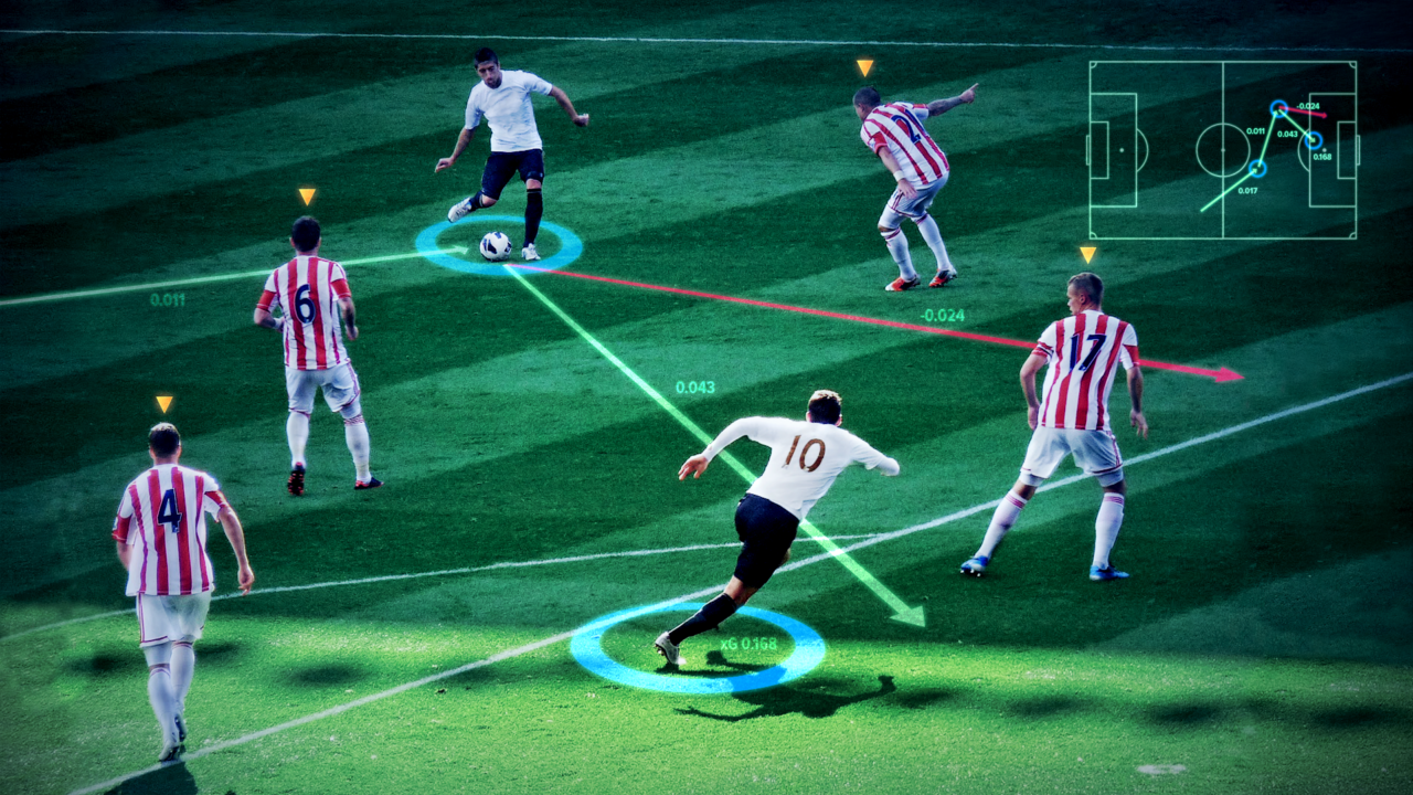
The performances of individual football players in games are hard to quantify due to the low-scoring nature of football. However, football analytics researchers and enthusiasts alike have proposed several football performance metrics for individual players in recent years.
Although the majority of these metrics focuses on measuring the quality of shots using expected-goals models, there has been an increasing interest in quantifying other types of individual player actions as well. In this blog, we introduce a novel approach to measure football players’ on-the-ball contributions from passes during games.
Our approach measures the expected impact of each pass on the scoreline. We value a pass by computing the difference between the expected reward of the possession sequence constituting the pass both before and after the pass. That is, a pass receives a positive value if the expected reward of the possession sequence after the pass is higher than the expected reward before the pass. Our approach employs a k-nearest-neighbor search with dynamic time warping as a distance function to determine the expected reward of a possession sequence. In the remainder of this blog, we guide you through the steps we took to develop our approach.
Data
We obtained game data for 9065 games in the English Premier League, Spanish LaLiga, German 1. Bundesliga, Italian Serie A, French Ligue Un, Belgian Pro League and Dutch Eredivisie via our partner Wyscout. For each of these games, our dataset contains play-by-play event data describing the most notable events that happened on the pitch. For each event, our dataset provides the following information: a timestamp (i.e., half and time), the team and player performing the event, the type (e.g., pass or shot) and subtype (e.g., cross or high pass), and the start and end location.
The table above shows an excerpt from our dataset showing five consecutive passes. Subtype 85 represents a simple pass, whereas subtype 80 represents a cross. The coordinates, which range from 0 to 100 in both directions, express the percentage distance across the width and length of the pitch. From the perspective of the goalkeeper playing for the team performing the action, the origin of the coordinate system is the nearest corner of the pitch to his left.
Approach
Valuing individual actions such as passes is challenging due to the low-scoring nature of football. Since football players get only a few occasions during games to earn reward from their passes (i.e., each time a goal is scored), we resort to computing the passes’ expected rewards instead of distributing the actual rewards from goals across the preceding passes. More specifically, we compute the number of goals expected to arise from a given pass if that pass were to be repeated many times. To this end, we propose a four-step approach to measure football players’ expected contributions from their passes during football games. We now discuss each of these four steps in turn.
Constructing possesion sequences
We split the event stream for each game into a set of possession sequences, which are sequences of events where the same team remains in possession of the ball. The first possession sequence in each half starts with the kick-off. The end of one possession sequence and thus also the start of the following possession sequence is marked by one the following events: a team losing possession (e.g., due to an inaccurate pass), a team scoring a goal, a team committing a foul (e.g., an offside pass), or the ball going out of play.
Labeling possesion sequences
We label each possession sequence by computing its expected reward. When a possession sequence does not result in a shot, the sequence receives a value of zero. When a possession sequences does result in a shot, the sequence receives the expected-goals value of the shot. This value reflects how often the shot can be expected to yield a goal if the shot were to be repeated many times. For example, a shot having an expected-goals value of 0.13 is expected to translate into 13 goals if the shot were to be repeated 100 times.
Valuing passes
We split each possession sequence into a set of possession subsequences. Each subsequence starts with the same event as the original possession sequence and ends after one of the passes in that sequence. For example, a possession sequence consisting of a pass 1, a pass 2, a dribble and a pass 3 collapses into a set of three possession subsequences. The first subsequence consists of pass 1, the second subsequence consists of pass 1 and pass 2, and the third subsequence consists of pass 1, pass 2, the dribble, and pass 3.
We value a given pass by computing the difference between the expected reward of the possession subsequence after that pass and the expected reward of the possession subsequence before that pass. Hence, the value of the pass reflects an increase or decrease in expected reward. We assume that a team can only earn reward whenever it is in possession of the ball. If the pass is the first in its possession subsequence, we set the expected reward of the possession subsequence before the pass to zero. If the pass is unsuccessful and thus marks the end of its possession subsequence, we set the expected reward of the possession subsequence after the pass to zero.
We compute the expected reward of a possession subsequence by first performing a k-nearest-neighbors search and then averaging the labels of the k most-similar possession subsequences. We use dynamic time warping (DTW) to measure the similarity between two possession subsequences. We interpolate the possession subsequences and obtain the x and y coordinates at fixed one-second intervals. We first apply DTW to the x coordinates and y coordinates separately and then sum the differences in both dimensions.
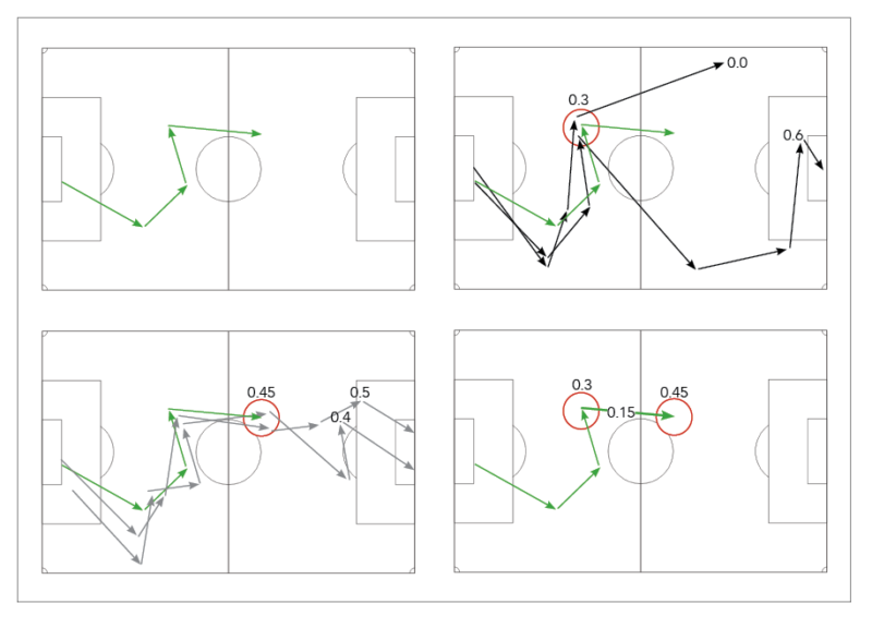
Visualization of our approach to value passes. In this example, we value the last pass of the possession sequence shown in green. We obtain a pass value of 0.15, which is the difference between the value of the possession subsequence after the pass (0.45) and the value before the pass (0.30)
The figure above shows a visualization of our approach for valuing passes. In this example, we aim to value the last pass in the possession sequence shown in green (top-left figure). First, we compute the value of the possession subsequence before the pass (top-right figure). We compute the average of the labels of the two nearest neighbors, which are 0.0 and 0.6, and obtain a value of 0.3. Second, we compute the value of the possession subsequence after the pass (bottom-left figure). We compute the average of the labels of the two nearest neighbors, which are 0.4 and 0.5, and obtain a value of 0.45. Third, we compute the difference between the value after the pass and the value before the pass to obtain a pass value of 0.15 (bottom-right figure).
Rating players
We rate a player by first summing the values of his passes for a given period of time (e.g., a game, a sequence of games or a season) and then normalizing the obtained sum per 90 minutes of play. We consider all types of passes, including open-play passes, goal kicks, corner kicks, and free kicks.
Results
We split the available data into three datasets: a train set, a validation set, and a test set. We respect the chronological order of the games. Our train set covers the 2014/2015 and 2015/2016 seasons, our validation set covers the 2016/2017 season, and our test set covers the 2017/2018 season.
We use the XGBoost algorithm to train the expected-goals model. After optimizing the parameters using grid search, we set the number of estimators to 500, the learning rate to 0.01, and the maximum tree depth to 5. We use the dynamic time warping implementation provided by the dtaidistance library to compute the distances between the possession subsequences. We set the number of nearest neighbors to 10, which we empirically found to be the optimal number for this task.
We now present the players who provided the highest on-the-ball contributions from their passes during the 2017/2018 season according to our approach. We first present an overall ranking and then present a ranking only showing players under the age of 21.
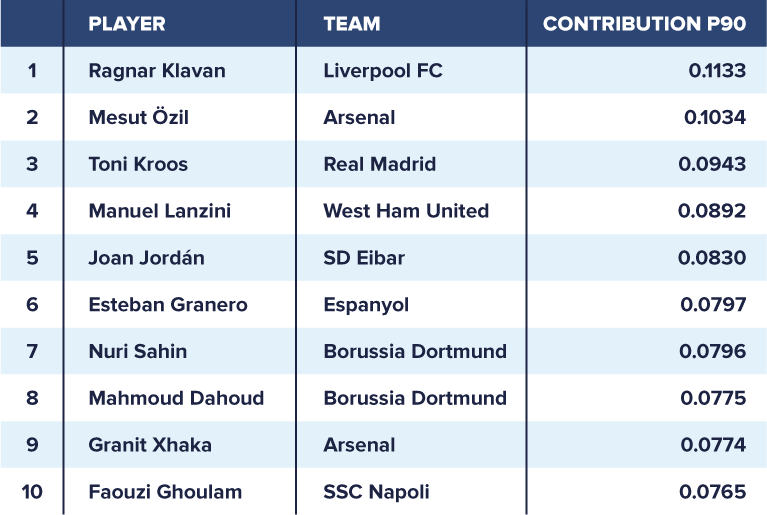
The table above shows the top-ten-ranked players who played at least 900 minutes during the 2017/2018 season in the English Premier League, Spanish LaLiga, German 1. Bundesliga, Italian Serie A, and French Ligue Un. Ragnar Klavan, who is a ball-playing defender for Liverpool FC, tops our ranking with an expected contribution per 90 minutes of 0.1133. Arsenal’s advanced playmaker Mesut Özil ranks second, whereas Real Madrid’s deep-lying playmaker Toni Kroos ranks third.
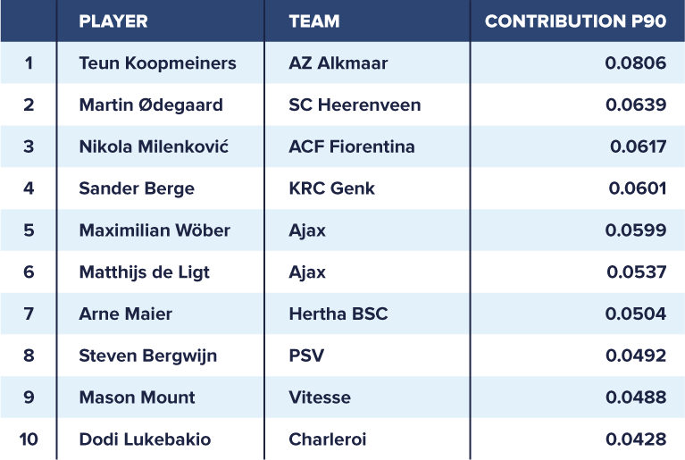
The table above shows the top-ten-ranked players under the age of 21 who played at least 900 minutes during the 2017/2018 season in Europe’s top-five leagues, the Dutch Eredivisie or the Belgian Pro League. Teun Koopmeiners (AZ Alkmaar) tops our ranking with an expected contribution per 90 minutes of 0.0806. Real Madrid-loanee Martin Ødegaard (SC Heerenveen) ranks second, whereas Nikola Milenković (ACF Fiorentina) ranks third.
Conclusion
This blog introduced a novel approach for measuring football players’ on-the-ball contributions from passes using play-by-play event data collected during games. While our approach is still under development and needs further polishing, our initial results presented above look very promising at the least.
JOIN US!
We always strive to attract the brightest (tech) talents in the world in order to create technological excellence


